Tricks to improve the performance of the CIFAR-10 classifier

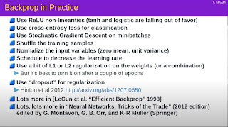
I participate in a weekly meeting with the TWIML (This Week in Machine Learning) group, where we go through the deep learning video lectures (with Pitorch) from the NYU (New York University) course. Each week we cover one of the lectures in a “flipped classroom” fashion – we watch the video ourselves before we participate, and one person leads the discussion, covering the main points of the lecture and moderating the discussion. Although this starts with the basics, I have found the discussions so far to be very insightful. Next week’s lecture is on Stochastic Gradient Descent and Backpropagation (Lecture 3) by Jan LeCun. At the end of the lecture, he lists some tricks for effectively training neural networks using back propagation.

To be fair, none of these tricks should be new information to people who train neural networks. Indeed, in Keras, most if not all of these tricks can be enabled by setting a parameter somewhere in your pipeline. However, this was the first time I had seen them listed in one place and I thought it would be interesting to test them with a simple network. This way, we can compare the effect of each of these tricks and more importantly for me, teach me how to do it using Pytorch.

The network I chose to do this with is the CIFAR-10 classifier, implemented as a 3-layer CNN (Convolutional Neural Network), with a structure identical to that described in the Tensorflow CNN Tutorial. The CIFAR-10 dataset is a dataset of approximately one thousand low-resolution (32, 32) RGB images. The nice thing about CIFAR-10 is that it is available as a canned dataset through the torch package. We explore the following scenarios. In all cases, we train the network using training images and validate at the end of each epoch using test images. Finally, we evaluate the trained network in each case using the test images. We compare the trained network using micro F1-scores (same accuracy) on the test set. All models were trained using the Adam optimizer, with the first two using a fixed learning rate of 1e-3 and the others using an initial learning rate of 2e-3 and exponential decay around 20% of epochs. All models were trained for 10 epochs with a batch size of 64.

1. basic — We include some suggestions in the slide, such as using a ReLU activation function on tanh and logistic, using a cross-entropy loss function (combined with Log Softmax as the final activation function), doing stochastic gradient descent on mini-patches, and interference. The training examples are already in their infancy as they are quite basic and their usefulness is not really in question. We also use Adam’s optimizer, based on Lekun’s comment during the lecture to prefer adaptive optimizers over the original SGD optimizer.
2. norm_inputs — Here we find the mean and standard deviation of the training set images, then scale the images in both the training and test sets by subtracting the mean and dividing by the standard deviation.
3. lr_schedule — In the previous two cases we used a fixed learning rate of 1e-3. Although we already use the Adam optimizer, which will give each weight its learning rate based on the gradient, here we also create an exponential learning rate graph that exponentially decays the learning rate at the end of each epoch. This is a built-in graph provided by Pytorch, along with several other built-in graphs.
4. weight_decomposition — Weight loss is better known as L2 regulation. The idea is to add a fraction of the sum of the squared weights to the loss and let the network minimize it. The net effect is to keep the weights small and avoid gradient blowup. The L2 adjustment is available to be set directly in the optimizer as a weight_decay parameter. Another related regularization strategy is L1 regularization, which uses the absolute value of the weights instead of the squared weight. L1 regularization can also be implemented using code, but is not directly supported (ie as an optimizer parameter) as L2 regularization is.
5. initial_weights — This is not listed in the slides, but is mentioned in LeCun’s Efficient Backprop paper (which is listed). Although by default module weights are initialized to random values, some random values ​​are better than others for convergence. Kaimeng (or He) activities are preferred for ReLU activation, which is what we used (Kaimeng Uniform) in our experiment.
6. abandoned_dense — Extractions can be placed after the activation functions, and in our network they can be placed after the activation function after the Linear (or dense) modulus or the convolutional modulus. Our first experiment places the Dropout module with probability 0.2 after the first Linear module.
7. dropout_conv — Dropout modules with a release probability of 0.2 are placed after each convolution module in this experiment.
8. abandon_both — Dropout modules with probability 0.2 are placed after both the convolution and the first linear module in this experiment.

The code for this exercise is available at the link below. It was run on a Colab (Google Colaboratory) (free) GPU instance. The Open in Colab button at the top of the notebook lets you launch it yourself if you want to explore the code.

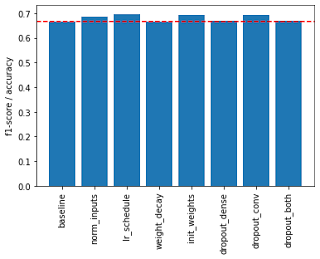
The notebook estimates and reports the precision, confusion matrix, and classification report (with per-class precision, recall, and F1-score) for each model listed above. Additionally, the bar chart below compares micro F1-scores across models. As you can see, input normalization (scaling) leads to better performance, and the best results are achieved using the learning rate schedule, weight initialization, and dropout implementation for convolutional layers.

That’s basically all I had today. The main benefit of the exercise for me was figuring out how to implement these tricks in Pytorch. I hope this will be useful as well.